The integral of the primary curve is usually obtained by treating the washout as being monoexponential (Hamilton et al., 1932). The empirical observation was made by Stow (1954) that the primary curve is lognormal in shape. We have found that the primary curve together with the first part of the secondary curve is closely approximated by a double lognormal plot - see figure. The lognormal approach to fitting the primary curve was not widely adopted possibly for two reasons: 1. At that time it was difficult to fit the function to the data. 2. There did not seem to be any theoretical justification. The function has many advantages. It seems more satisfactory to use as much of the curve representing the data as possible to estimate the tail of the primary curve. It is robust and extremely effective at handling slightly noisy data. We have previously produced both theoretical and experimental evidence in support of Stow's observation and developed an equation for deriving the integral of a lognormal from the first part of the curve (Linton et al., 1995). We showed that for a set of swirl chambers in series (assuming that the chambers are identical, that the indicator is injected at the upstream end instantaneously, that there is perfect mixing and that there is a constant flow into and out of each chamber) the transfer function would produce an indicator dilution curve which would be the same shape mathematically as the chi squared distribution with n/2 degrees of freedom. Over the usual range of sigma (the measure of skewness) for primary indicator dilution curves, the difference between the chi squared and corresponding lognormal integrals is less than 2%. Lognormal curves with different values of sigma are shown in the figure.
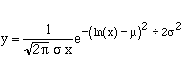
A variable has a lognormal distribution if the logarithm of the variable is normally distributed. The probability density function of the lognormal distribution is:
where mu and sigma are the mean and standard deviation respectively of the normal distribution from which the logarithmic transformation was obtained. The equation we have used to model indicator dilution curves is:
![]()
The parameters in this equation allow the curve to be scaled horizontally (mu) and vertically (alpha), to be shifted along the time axis (To), and to be changed in terms of skewness (sigma).
The lognormal is derived as follows:
Area A = integral from start of curve to 98% of peak value on ascending limb
Area B = integral from 98% of peak on ascending limb to 70% of peak on descending limb
The parameters of the lognormal are calculated from these two areas as follows:

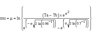
where Ta is the cut-off time for area A and Tb is the cut-off time for area B
![]()
![]()
The error of the integral of a lognormal curve calculated as above is less than 0.05%. Inspection of hundreds of curves showed that recirculation is extremely unlikely to occur before the 70% cutoff (except during hard exercise).
The fitted lognormal has the same areas A and B as the data and so when fitting the lognormal to the data any error is concentrated in the tail of the curve or area C , which is the integral of the lognormal minus areas (A+B). The secondary curve should be represented by the difference between the lognormal and the original curve. Sometimes the secondary curve does not look 'right' and may even be 'double-humped' - see figure. This is obviously wrong and implies that the tail of the primary curve is not always accurately described by the tail of the lognormal. To address this problem of variation in the tail of the primary curve, we have used an iterative method to fit an exponential to the part of the curve after the 70% cut-off. We increase area C by a factor of 1.5 (C factor) and plot it as a monoexponential. The integral of this exponential is then decreased until all the points on the original curve between 70% and 30% of peak lie to the right of (or coincide with) this exponential, or until the C factor=1. When the data shown in the previous figure is reanalysed using this modification the secondary curve loses the early hump - see figure. A typical patient curve has a C factor of 1.2 which represents an approximate 5% increase in the calculated area of the whole curve. In practice there is no single function that can represent the dilution curve perfectly in all cases. The advantage of using the lognormal to determine the limits of the integral of the monoexponential is that the algorithm cannot produce a 'wild' value. In this current algorithm we have in a sense combined the best features of the Stow lognormal approach with the original Hamilton monoexponential extrapolation and may be as close as one can get to the truth. There appears to be a small variation in the final washout of indicator from the lungs.